 |
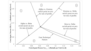
| Figure 1: Partitions For A Parameter Space |
This post extends this
and this.
I am considering perturbations of coefficients of production in a numerical example of the recurrence
of truncation without the reswitching of techniques.
The example consists of two industries that produce new machines and corn, respectively. The physical life of a machine
is two years in each industry. Corn acts as circulating capital, as well as the consumption good.
As the result of technical change, coefficients of production vary. No variation in labor coefficients or of
the output matrix are considered here so as to retain forward substitution of labor in the corn industry at the switch point between Alpha and Gamma and reverse labor substitution at the switch point between Beta and Delta.
Accordingly, I consider permutations of the coefficients of production in the first row of the input matrix.
These coefficients of production specify inputs of circulating capital for each process, when operated
at unit level.
Previously, I considered
perturbations of the pair of coefficients that specify the inputs of corn needed for each machine when
the machine is run in the second year of its life.
Today, I consider perturbations in a1,1 and a1,3, the coefficients that specify
the inputs of corn needed for each machine when
the machine is run in the first year of its life.
Figure 1, at the top of this post, partitions a part of the parameter space. In drawing this figure,
a1,2 = 0.635 and a1,4 = 0.319. Each partition corresponds to a fluke switch point.
For the values of a1,2 and a1,4 in Table 1 in
this post,
the parameters corresponding to the fluke switch point in which the four wages curves intersect on the axis for the rate of profits is an economically meaningless point in the second quadrant.
A switch point is a fluke if it is a knife edge case in which almost all perturbations of model
parameters destroy its defining properties. Four of the five partitions correspond to a switch point
on the axis for the rate of profits. With four techniques, switch points between six pairs are possible.
A switch point between Alpha and Delta can only occur as an intersection of all four curves. The same goes for a
switch point between Beta and Gamma. These two pairs of techniques correspond to the partition for the
switch point at which all four wage curves intersect.
The sequence of techniques along the wage frontier is invariant in each numbered region in the slice of the
parameter space in Figure 1.
Table 1 lists the cost-minimizing techniques in each region, in order of an increasing rate of profits.
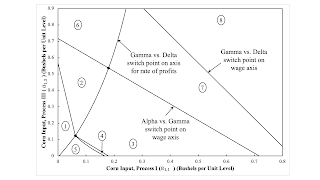
Other partitions, depicted in Figure 2, exist up and to the right.
One is for a switch point between Alpha and Gamma on the wage axis, and another is for the switch point between
Gamma and Delta on the wage axis. Three new regions are associated with these partitions. Gamma is cost-minimizing,
whatever the distribution of income, for a high enough value of a1,3, not exceeding unity,
in the upper left. Delta is cost-minimizing alone in a region to the northeast. Gamma and Delta are cost-minimizing,
in that order for an increasing rate of profits, in a region bounded below by region 3 and also by these two additional regions.
| Region | Techniques | Notes |
| 1 | Alpha | No switch point. |
| 2 | Alpha, Gamma | Lower rate of profits associated with truncation in corn industry, greater output per worker. |
| 3 | Alpha, Gamma, Delta | Lower rate of profits associated with truncation, greater output per worker. |
| 4 | Alpha, Gamma, Delta, Beta | Recurrence of truncation in corn industry. |
| 5 | Alpha, Beta | Lower rate of profits associated with truncation in machine industry, greater output per worker. |
| 6 | Gamma | No switch point. |
| 7 | Gamma, Delta | Lower rate of profits associated with truncation in corn industry, greater output per worker. |
| 8 | Delta | No switch point. |
 |
| Figure 2: An Expanded View of Partitions For A Parameter Space |
Suppose technical change lowers corn inputs for the first year a machine is operated, in either industry,
while leaving all other coefficients of production unchanged. Some trajectories going roughly from
the northeast to the southwest in Figures 1 and 2 cross through region 4. Under this specific
form of technical progress, the recurrence of truncation can arise and then disappear in secular time. But it need not.