Introduction: Why Monetary Policy Needs a Firm Theoretical Foundation
Monetary policy is fundamentally about stabilising nominal spending — nominal GDP — to support economic growth and maintain price stability.
For the euro area, this challenge is particularly complex given structural differences across member states, asymmetric shocks, and the unique institutional arrangement of monetary union without fiscal union.
Traditional frameworks have largely relied on interest rate rules — most notably the Taylor rule — which use inflation and output gaps as policy guides.
Whilst these rules have been influential, they often fail to account for the inherent instability and variability of money demand, potentially creating misalignments between policy settings and economic fundamentals.
The McCallum rule offers a theoretically robust alternative, firmly grounded in the quantity theory of money and nominal income targeting.
It provides a transparent, quantity-based framework for monetary policy that explicitly accounts for fluctuations in money velocity — a critical consideration in the euro area context.
The Origins and Development of the McCallum Rule
Bennett McCallum, the Carnegie Mellon economist who sadly passed away in 2024, developed his eponymous rule in the late 1980s as a direct response to the perceived shortcomings of both discretionary monetary policy and simple monetary targeting.
His seminal 1988 paper “Robustness Properties of a Rule for Monetary Policy” (Carnegie-Rochester Conference Series) introduced the rule as a way to operationalise nominal GDP targeting through monetary base control.
McCallum’s motivation was straightforward: whilst Friedman’s k-percent rule assumed stable velocity, and Taylor’s (1993) rule relied on difficult-to-measure output gaps, a rule that explicitly adjusted for velocity trends could provide more reliable guidance.
His subsequent work, particularly “Alternative Monetary Policy Rules: A Comparison with Historical Settings for the United States, the United Kingdom, and Japan” (NBER, 1999), demonstrated the rule’s superior performance across different monetary regimes.
The rule gained some attention during the 2008 crisis when interest rate rules hit the zero lower bound.
McCallum himself argued in “Nominal GDP Targeting” (Shadow Open Market Committee, 2011) that his quantity-based approach remained viable even when conventional interest rate policy became impotent.
The ECB’s Historical Relationship with Monetary Aggregates
It’s worth noting that the ECB began its operations with an explicit monetary pillar, including a reference value for M3 growth of 4.5% annually.
This two-pillar strategy — combining monetary analysis with economic analysis — reflected the German Bundesbank tradition and recognised the long-run relationship between money growth and inflation.
The ECB’s original M3 reference value was derived from the quantity equation itself: 2% inflation target plus trend real GDP growth (2-2.5%) minus trend velocity decline (0.5-1%). This was essentially a simplified McCallum rule without the feedback mechanism.
However, the ECB progressively downgraded the role of monetary analysis, particularly after 2003, citing velocity instability and the weak short-run relationship between money growth and inflation.
This abandonment of monetary analysis was in my view a grave error. By throwing out the monetary baby with the bathwater, the ECB deprived itself of crucial information about monetary conditions.
As the analysis below will demonstrate, the ECB’s neglect of monetary aggregates led to systematic policy errors: excessive M3 growth prior to 2008 (contributing to asset bubbles and imbalances) followed by a prolonged period of undershooting that hampered the recovery and kept inflation persistently below target.
Had the ECB paid proper attention to monetary aggregates and nominal spending growth — as the McCallum rule prescribes — these costly errors could have been avoided.
The McCallum rule, by explicitly incorporating velocity trends and feedback from nominal GDP, addresses precisely the shortcomings that led the ECB to abandon its monetary pillar. Rather than abandoning monetary analysis when velocity became unstable, the ECB should have adopted a more sophisticated framework that accounts for velocity changes.
The Quantity Theory of Money and Nominal Income Targeting
The McCallum rule builds on the classical equation of exchange:
M × V = P × Y
Where:
- M is the money supply
- V is velocity
- P is the price level
- Y is real output
In growth terms, this becomes:
Δm + Δv = Δp + Δy = Δx
Where:
- Δm is money supply growth
- Δv is velocity growth
- Δp is inflation
- Δy is real GDP growth
- Δx is nominal GDP growth
The key insight is that stable nominal GDP growth ensures balanced growth in real output and prices. Monetary policy’s role, therefore, is to adjust money supply growth to offset velocity fluctuations and guide nominal GDP toward its target path.
The McCallum Rule Formalised
Building on this framework, McCallum proposed a systematic policy rule:
Δmₜ = -vₜ + xₜ + λ(x*ₜ – xₜ)
Where:
- v*ₜ is the trend velocity growth — recognising that velocity is not constant but evolves structurally over time due to financial innovation, regulation, and behaviour
- x*ₜ is the target nominal GDP growth, set by the inflation target plus trend real output growth
- xₜ is actual nominal GDP growth
- λ is a policy reaction coefficient, modulating responsiveness to deviations from target
This rule has several compelling features:
First, it provides direct control over nominal spending. By targeting money growth to stabilise NGDP, the rule ensures policy responds to the key macroeconomic aggregate affecting economic activity.
Second, it incorporates velocity trends. Unlike the ECB’s abandoned fixed reference value, it adjusts for persistent shifts in money demand — crucial for modern economies where velocity exhibits some structural changes.
Third, the systematic feedback mechanism λ(x*ₜ – xₜ) enables proportional policy responses to deviations in nominal income growth, providing automatic stabilisation.
Why Use M3 Instead of the Monetary Base?
McCallum’s original formulation targeted the monetary base — reserves and currency directly controlled by the central bank. The base represents the foundation of money creation and is under tight central bank control.
However, in the euro area context, the monetary base is relatively small compared to broader aggregates, and its relationship with nominal GDP has become increasingly unstable, particularly during unconventional monetary policy episodes such as quantitative easing. As McCallum himself acknowledged in later work (see “Theoretical Analysis Regarding a Zero Lower Bound on Nominal Interest Rates,” Journal of Money, Credit and Banking, 2000), the choice of monetary aggregate matters for practical implementation.
For empirical implementation, I therefore use M3 — the broadest monetary aggregate — which better captures the liquidity available to the economy and the monetary conditions affecting spending decisions.
This choice is particularly appropriate given the ECB’s historical focus on M3 and the extensive data available for this aggregate.
The trade-off is clear: M3 velocity is less directly controllable than base velocity, requiring careful estimation of velocity trends (hence our 10-year moving average approach) and interpretation of the McCallum rule as a policy benchmark rather than a mechanical target.
Empirical Implementation: Estimating Trends
Applying the McCallum rule requires careful estimation of trend velocity growth (v*ₜ) and trend real GDP growth (y*ₜ).
I employ 10-year rolling averages of quarterly growth rates, which smooth cyclical fluctuations whilst capturing gradual structural changes.
This methodology follows McCallum’s own empirical applications, where he typically used moving averages of 12-16 quarters to estimate velocity trends.
The inflation target π* is set at 2% annually (approximately 0.5% quarterly), consistent with ECB objectives.
The reaction coefficient λ is calibrated at 0.5, reflecting the balanced responsiveness recommended in McCallum’s original work and subsequent empirical studies.
To account for uncertainty, I incorporate bands of ±1 standard deviation of velocity growth. For the extreme 2020-22 COVID period, I fix the band width at pre-pandemic levels to prevent distortion from these exceptional circumstances.
This framework provides a theoretically grounded, empirically implementable guide for monetary policy — one that respects the fundamental relationships between money, velocity, and nominal income whilst remaining flexible enough to accommodate the complexities of modern monetary economics.
It represents what the ECB’s two-pillar strategy should have evolved into, rather than being unceremoniously abandoned. The cost of that abandonment — in terms of excessive monetary growth pre-2008 and persistent undershooting thereafter — has been substantial.
Historical Review Through the McCallum Lens: A Detailed Narrative
The journey of euro area monetary policy since the launch of the single currency in 1999 reveals a story of evolving challenges, shifting economic realities, and the consequences of abandoning systematic monetary analysis.
By examining actual monetary growth relative to the McCallum rule’s prescriptions, we gain a revealing window into how policy decisions aligned — or more often diverged — from theoretically grounded benchmarks designed to stabilise nominal GDP.
The Early Years (2000–2005): Caution and Relative Stability
The birth of the euro marked a historic moment. The ECB was navigating uncharted waters, crafting a monetary regime for a diverse economic union. During these formative years, the graph below reveals a reassuring picture: the orange line of actual M3 growth oscillated closely around the red dashed McCallum target, mostly staying within the grey uncertainty bands.
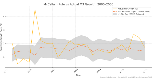
This alignment was no accident. The ECB still maintained its two-pillar strategy, with the monetary pillar providing discipline. When M3 growth briefly spiked above 4% in 2001, it quickly corrected back toward the 2% target range. The central bank was effectively following a McCallum-type rule, even if not explicitly.
This period demonstrates what monetary policy can achieve when it respects monetary aggregates and nominal income dynamics. The relative stability wasn’t luck — it was the result of systematic policy grounded in sound monetary principles.
The Expansion and Overheating Phase (2005–2008): The Prelude to Crisis
From 2005 onwards, the graph below tells a dramatically different story. The orange line of actual M3 growth breaks decisively above the McCallum target, repeatedly piercing the upper uncertainty band. By 2007, M3 growth was consistently running at 3% or higher — well above the rule’s prescription of around 2%.
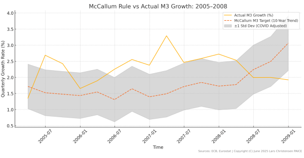
This wasn’t a brief deviation but a sustained period of monetary excess. The ECB had by then effectively abandoned its monetary pillar, dismissing the warning signals from accelerating money growth.
During this period instead of focusing on M3 growth and nominal spending growth the ECB got fooled by an excessive focus on actual inflation that in the early stage of the period still remained fairly low and stable.
The graph shows the consequences: a widening gap between actual policy and what systematic nominal income targeting would have prescribed.
The McCallum rule would have called for tightening — reducing M3 growth back toward the 2% level.
Instead, the ECB maintained an accommodative stance, flooding the euro periphery with excess liquidity that fuelled housing bubbles and unsustainable debt accumulation.
The Crisis and Austerity Period (2008–2014): The Cost of Overcorrection
The 2008 crisis marks a dramatic inflection point on the graph. The orange line plummets from above 3% to below -1% by 2010, crashing through the lower uncertainty band.
While the McCallum rule (red dashed line) called for maintaining positive money growth around 1-2% to offset collapsing velocity, actual policy went in the opposite direction.
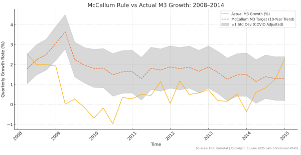
This visual evidence is damning. For nearly five years, from 2010 to 2014, actual M3 growth remained below — often far below — what the McCallum rule prescribed. The ECB was actively tightening monetary conditions during the deepest recession since the 1930s.
This is the crucial insight that the interest rate lens obscures. Yes, the ECB cut rates — but not nearly enough to offset the velocity collapse and generate the money growth required to stabilise nominal GDP.
The McCallum rule shows what should have happened: a significant expansion of M3 to compensate for plummeting velocity. Instead, M3 growth turned sharply negative.
This analysis reveals the tragedy of discretionary policy without a nominal income anchor. While the rule called for support, the ECB delivered austerity. The prolonged period below the lower band corresponds exactly with the euro area’s double-dip recession and lost decade.
The Recovery and Quantitative Easing Era (2015–2019): Gradual Realignment
The launch of Quantitative Easing (QE) in 2015 shows up clearly on the graph below. The orange line rises from negative territory back toward the McCallum target.
For the first time since the crisis in 2008, actual M3 growth converges with the rule’s prescription, oscillating around the 1% level within the uncertainty bands.
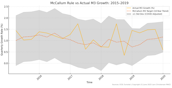
This visual convergence tells the story of belated recognition. The ECB had finally acknowledged (at least indirectly) that monetary aggregates matter and that supporting nominal income requires adequate money growth.
The graph validates what monetarist critics like myself had argued for years — proper monetary expansion was needed and, when finally delivered, it worked.
The Pandemic Shock and Response (2020–2021): Learning from Past Mistakes
The COVID period reveals a dramatic but ultimately vindicated policy response from the ECB as the graph below show.
The orange line (actual M3 growth) initially plunges to -11% in early 2020 as the pandemic struck, before surging to an extraordinary peak of 12% by mid-2020. The red dashed line (McCallum target) shows a more moderate pattern, rising from 3% to about 6% before falling to -4%.
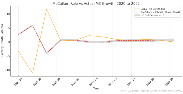
The divergence is revealing. While actual M3 growth swung wildly — from -11% to +12% — the McCallum rule prescribed a much more measured response. When the pandemic hit and M3 growth collapsed to -11%, the rule was already signalling the need for expansion to around 6%.
As the ECB responded with massive stimulus, pushing M3 growth to 12%, the McCallum rule was already moderating, recognising that velocity was rebounding.
The crucial insight comes from examining the full period.
From 2020 to end-2022, the average quarterly M3 growth was approximately 0.41%, while the McCallum rule target averaged 0.71%. This means that despite the dramatic spike in 2020, the ECB’s overall monetary stance was actually more restrictive than what the rule prescribed.
This finding challenges the conventional wisdom — including my own initial assessment — that ECB policy had also become too easy during the pandemic, albeit less so than in the US.
The McCallum rule reveals a different story: the ECB’s monetary stance was actually tighter than “optimal” throughout the COVID period – at least compared to the McCallum rule.
This restraint becomes even clearer when compared to the Fed. While euro area M3 growth peaked at 12% year-on-year in 2021, US M2 growth reached an astonishing 25%. The ECB provided necessary crisis support but avoided the Fed’s monetary excess.
The inflation comparison graph below tells the story even more starkly. US inflation (red line) began accelerating sharply in early 2021, rising from near zero to over 5% by mid-year.
Crucially, US inflation had already reached nearly 9% by February 2022 — before Russia’s invasion of Ukraine — and was clearly on an upward trajectory driven entirely by domestic monetary and fiscal excess.
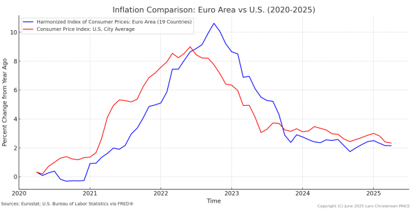
In sharp contrast, Euro area inflation (blue line) remained subdued relative to the US throughout 2021. But as war fears escalated in early 2022 in Europe inflation started to accelerate in the euro area.
While US inflation was already near its peak when the war began, European inflation shot up from 5% to over 10% in the months following the invasion. This timing difference is decisive evidence that US and European inflation had fundamentally different causes.
The graph reveals clear evidence of US monetary policy “leading” European inflation. The red line consistently runs 6-12 months ahead of the blue line throughout the cycle.
As US inflation accelerated through 2021, European inflation began a modest rise in late 2021 — consistent with spillovers from American monetary excess but nothing like the surge that would follow the war. When US inflation peaks at 9% and begins declining in mid-2022, European inflation continues rising to its 10.6% peak several months later.
This leadership pattern indicates significant spillover effects, but the magnitude tells the real story.
Before Ukraine, Europe was experiencing perhaps 2-3 percentage points of imported inflation from easy US monetary conditions. But the explosion from 5% to over 10% inflation came only with the war — a pure supply shock that the ECB could not (and should not) have prevented regardless of policy stance.
The fact that European M3 growth averaged below the McCallum target throughout this period confirms that European inflation was to a large extent supply-side driven (from 2022) — a consequence of war and energy shocks, with some imported US inflation primarily in 2021, rather than domestic monetary excess. The US, having already reached 9% inflation before any war effects, was clearly experiencing a classic demand-driven inflation that the Fed had created through excessive stimulus.
The Post-Pandemic Period and Recent Tightening (2021–2025): From Convergence to Renewed Risks
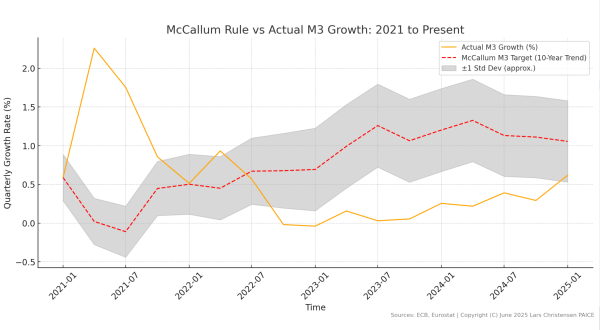
The graph below shows that through 2021, actual M3 growth in the euro area declines sharply to around 0.5%, converging with the rising McCallum target.
By late 2021 and into 2022, both lines track closely together between 0.5% and 1%, with actual policy closely matching what the rule prescribed.
During this period, the ECB maintained its deposit rate at -0.50%, providing continued support as the economy recovered.
This convergence vindicated both the ECB and the McCallum framework.
By moderating M3 growth from its pandemic peak while keeping it aligned with the rule’s prescription, the ECB avoided the Fed’s error of maintaining excessive stimulus.
However, the Fed’s procrastination in addressing its own inflation — keeping rates at zero until March 2022 despite inflation exceeding 5% by mid-2021 — created spillovers that complicated the European picture.
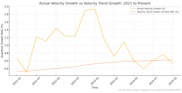
The velocity graph below illustrates the mechanism of these spillovers.
From early 2021, actual velocity growth (orange line) surges dramatically above its trend (red dashed line), jumping from 0.3% to over 1.2% by late 2021.
This acceleration continues through 2022, with velocity growth peaking near 2% — more than triple its trend rate of around 0.5%.
This surge in velocity reflects rising inflation expectations imported from the US, as markets anticipated that global inflation pressures would eventually reach Europe.
These US spillovers lifting velocity above trend present a genuine dilemma: when velocity rises due to imported expectations rather than domestic conditions, central banks must balance competing risks.
Some of the surge in velocity likely also have to be seen in the light of the communication from the ECB that during 2021 continued to signal a very easy monetary stance despite the need to normalise montary conditions.
The extraordinary gap between actual and trend velocity growth in 2022-2023 shows the magnitude of this external shock that the ECB had to navigate.
When inflation did surge in Europe following Russia’s invasion, it was overwhelmingly driven by war and energy shocks rather than monetary excess. The ECB raised the deposit rate from -0.50% to 4.00% by September 2023 — 450 basis points in 14 months. This aggressive response needs to be understood in the context of velocity running far above trend, providing additional monetary stimulus that needed offsetting.
The M3 growth graph shows actual M3 growth plunging to near zero from mid-2022, remaining there through 2023, consistently below the McCallum target.
However, this apparent tightness must be viewed alongside the velocity surge — the combination of near-zero M3 growth and velocity running 1-1.5 percentage points above trend meant the ECB was striking a reasonable balance between competing objectives.
By late 2023, the velocity graph shows a sharp reversal, with actual velocity growth plunging below trend and even turning negative in 2024.
This normalisation of velocity — from 2% back toward the 0.6% trend — justified the ECB’s decision to begin cutting rates.
The fact that M3 growth has started recovering, albeit gradually, suggests the ECB is managing the transition reasonably well.
Looking at both graphs together, the ECB appears to have navigated an extraordinarily difficult period with reasonable skill.
They avoided the Fed’s error of excessive stimulus, responded appropriately to the velocity surge driven by imported expectations, and began easing as velocity normalised.
While M3 growth remains somewhat below the McCallum target, this may reflect appropriate caution given the unprecedented nature of the shocks.
The ECB’s response — raising rates aggressively when velocity surged, then cutting as it normalised — represents a sensible application of the McCallum framework’s insights while adapting to exceptional circumstances.
The lesson is that even good policy rules require judgment in their application. The ECB’s performance during this period, while not perfect, demonstrates that systematic monetary policy based on nominal income targeting principles can successfully navigate even extreme external shocks and imported inflation expectations.
Where We Stand Today (June 2025): A Return to Equilibrium
As of June 2025, the euro area monetary landscape presents a remarkably different picture from the turbulence of recent years.
The annualised velocity and real GDP growth graphs below show a striking convergence: actual values (orange lines) have returned to almost perfect alignment with their long-term trends (red dashed lines), with both now comfortably within their ±1% uncertainty bands.
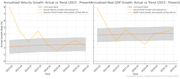
The velocity graph shows the dramatic journey from early 2023, when annualised velocity growth exceeded 8%. This has now normalised to around 2.5%, virtually identical to its 10-year trend. ‘
The sharp decline from the 2023 peak through mid-2024 represented the unwinding of inflation expectations, and the current stability within the grey band suggests these extraordinary monetary disturbances have finally worked through the system.
Similarly, the real GDP growth graph reveals the economy’s path from the volatile swings in 2020-2022 to a steady convergence around the 4% trend rate.
The wild oscillations of the recovery period have given way to stable growth, with actual GDP expansion now tracking its long-term potential. The absence of any significant deviation from the trend band indicates the economy is operating at equilibrium, neither overheating nor underperforming.
This dual convergence is crucial for monetary policy. When both velocity and real growth align with their long-term patterns — as they clearly do now — the McCallum rule provides its most reliable guidance.
With v = v* and y = y*, the fundamental drivers of nominal GDP are at their structural levels.
The ECB just cut the deposit rate by 25bp to 2.00% last week as expected, and market pricing suggests only one more 25 basis point cut in the coming months.
This cautious market expectation appears well-calibrated. With M3 growth now tracking the McCallum rule target, velocity at trend, and real growth at potential, the ECB is approaching neutral territory. Following the market’s guidance — one more modest cut to 1.75% — would likely achieve the appropriate stance.
This represents a remarkable achievement. After navigating extreme velocity swings from -1% to 8%, managing imported inflation from US policy errors, and weathering an energy crisis, the ECB has engineered a soft landing with all key variables converging to their equilibrium values.
The current alignment — M3 growth matching the McCallum target, v = v*, y = y* – suggests monetary policy is almost perfectly calibrated.
The lesson is clear: systematic monetary policy works.
Conclusion: The Visual Verdict and the Path Forward
A single graph can capture a quarter century of the euro area’s monetary policy journey—its successes, its missteps, and its crucial lessons.
The black line in the graph below represents the McCallum gap – the difference between actual M3 growth and the McCallum rule – while the red shaded area highlights medium-term trends through the 1-year centered moving average of this cap.
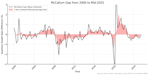
Periods where the gap remains close to zero—such as 2000-2005 and 2015-2019—reflect times when the ECB’s policy aligned closely with systematic principles, corresponding with economic stability and recovery.
Conversely, sharp deviations—excessive money growth from 2005 to 2008 and undershooting from 2009 to 2014—map precisely onto the eurozone crises.
The message is unmistakable: adherence to a rule-based framework akin to the McCallum rule fosters economic prosperity.
Departures into discretionary, untethered monetary expansions or contractions bring turmoil. This graph is far more than a historical record—it’s a clear indictment of the costs borne by abandoning systematic monetary policy, and simultaneously a roadmap for reform.
The pandemic years stand as a notable exception, where discretion arguably outperformed rigid rule-following – but even then, success hinged on embracing the McCallum spirit: adjusting appropriately to unprecedented uncertainty without the Fed’s overreach.
This exception, in fact, underscores the rule’s validity: systematic nominal income targeting delivers superior outcomes compared to unanchored discretion.
Now, as we approach equilibrium in mid-2025, with M3 growth aligned with targets, velocity and real growth steady on trend, and inflation near 2%, the moment is ripe for institutional reform.
As I have long argued, the ECB must adopt a comprehensive framework that remains within the inflation targeting mandate but is underpinned by:
- Systematic M3 growth guidance based on the McCallum rule, ensuring a quantity anchor in monetary policy
- Explicit monitoring of nominal GDP growth to align policy with sustainable nominal spending
- Ongoing market-based expectation analysis for real-time feedback on policy credibility
Had this framework been in place over the last 25 years, many policy errors could have been avoided.
The evidence is overwhelming: monetary aggregates matter, nominal income is the critical benchmark, and rules systematically outperform discretion.
The current alignment of key indicators presents the perfect opportunity to institutionalise these lessons.
Rather than waiting for the next crisis to expose the limits of pure inflation targeting, the ECB should act now and embrace the framework history demands.
The McCallum rule has proven its worth time and again. It’s time to make it a cornerstone of the ECB’s official toolkit.
Finally, if you would like to test the McCallum rule yourself, I have developed a ‘McCallum Rule Calculator’ where you can input different values for the variables in the McCallum rule. Try the Calculator here.